AI/ML Development Intro: Part 1
What is this?
I work in close proximity to a lot of AI/ML/big data engineers and have friends who are of the same variety. I somewhat understand the basic concepts of a neural network and I have some knowledge of vectors etc. but I’m tired of being the one left confused when having conversations… So, my plan is to get stuck in a little.. at least to train something and to work my way into a problem enough that I get confused.. and then end up with more of an understanding/appreciation as a result of it.
I had a quick look at some tutorials, the MNIST handwritten digit recognition being a common one. BUT, I didn’t like the amount of hand-holding, e.g.:
from sklearn.datasets import load_digits; digits = load_digits(),(x_train, y_train), (x_test, y_test) = mnist.load_data()
So I’m going to work-through several different tutorials:
- https://medium.com/@santiagu.gap/uncovering-the-magic-1-c1c7e23f836a
- https://www.toptal.com/developers/data-science/machine-learning-number-recognition
- https://www.geeksforgeeks.org/machine-learning/handwritten-digit-recognition-using-neural-network/
- https://www.digitalocean.com/community/tutorials/how-to-build-a-neural-network-to-recognize-handwritten-digits-with-tensorflow
- https://www.toptal.com/developers/data-science/machine-learning-number-recognition
- Some conversations with ChatGPT
The goal is to write down my version, with no stones left unturned.
Definitions
I’d heard a lot about various tools, but didn’t know exactly what they were, so:
- Jupyter (well, not new, but will be part of the stack)
- An interactive environment where you can write Python code, run it piece by piece, see outputs immediately, and add notes or visualizations.
- Notebook: interactive, cell-based interface
- Lab: more full-featured, like an IDE for notebooks
- Basically treated as you would you laptop/local IDE, used for development and development building/training, but not used for production (training OR inference)
- TensorFlow/Pytorch: Both ML frameworks - TensorFlow written by Google, Pytorch by Facebook. If I have time, I will try to develop using both of these, starting with tensorflow
- Airflow: A workflow orchestration tool for complex tasks. E.g. data preprocessing, training, evaluation, deployment
- DAG: Directed Acyclic Graph, basically steps in a multi-stage job that have dependencies on one-another, with tasks as “nodes” and edges meaning dependencies.
- MLFlow: A tool for experiment tracking, model versioning, and deployment.
- This can host models in it’s built-in registry
- Can serve models (production-ready)
My Stack
So I wanted a little bit of each of these layers, so I decided to run Jupyter Lab and Airflow inside docker.
I wanted to expose Airflow to Jupyter, so my DAGs could be written/triggered from the notebook.
Setup
I’m always conscious about installing anything on my macbook.. I can count the number of applications installed in homebrew on one hand. I generally use decontainers for absolutely everything - but this doesn’t really work for interacting with the Macbook’s Metal. After some thought (and discussion), I decided to use common AI/ML tooling on top of docker on another host.
This will be more similar to “real life” (or at least from my point of view within BigCorp) since everything is hosted in the cloud.
Setting up a basic docker-compose looks like:
version: "3.9"

services:
  postgres:
    image: postgres:15
    container_name: airflow_postgres
    restart: always
    environment:
      POSTGRES_USER: airflow
      POSTGRES_PASSWORD: airflow
      POSTGRES_DB: airflow
    volumes:
      - postgres_data:/var/lib/postgresql/data
    ports:
      - "5432:5432"
  airflow:
    image: apache/airflow:2.8.3-python3.11
    container_name: airflow
    restart: always
    environment:
      # Set UID to align with Jupyter
      AIRFLOW_UID: 50000
      AIRFLOW__CORE__EXECUTOR: LocalExecutor
      AIRFLOW__CORE__LOAD_EXAMPLES: False
      AIRFLOW__CORE__DAGS_FOLDER: /opt/airflow/workspace/dags
      # AIRFLOW__WEBSERVER__AUTH_BACKEND: "airflow.api.auth.backend.basic_auth"
      AIRFLOW__WEBSERVER__SECRET_KEY: "supersecret"
      AIRFLOW__DATABASE__SQL_ALCHEMY_CONN: postgresql+psycopg2://airflow:airflow@postgres:5432/airflow
    user: "${AIRFLOW_UID:-50000}"
    volumes:
      - ./workspace:/opt/airflow/workspace  # Shared DAGs/workspace
      - airflow_logs:/opt/airflow/logs  # Airflow logs persisted
    ports:
      - "8080:8080"  # Airflow web UI
    command: >
      bash -c "airflow db init &&
               airflow scheduler &
               airflow webserver"
    # deploy:
    #   resources:
    #     reservations:
    #       devices:
    #         - driver: nvidia
    #           capabilities: [gpu]  # Optional GPU passthrough

  jupyter:
    image: jupyter/datascience-notebook:latest
    container_name: jupyterlab
    restart: always
    environment:
      # Align UID with Airflow, just to help with file permissions
      NB_UID: 50000
      JUPYTER_ENABLE_LAB: "yes"
    volumes:
      - ./workspace:/home/jovyan/work  # Shared workspace
    ports:
      - "8887:8888"
    command: start-notebook.sh --NotebookApp.token='' --NotebookApp.password=''
    # deploy:
    #   resources:
    #     reservations:
    #       devices:
    #         - driver: nvidia
    #           capabilities: [gpu]  # Optional GPU passthrough

volumes:
  airflow_logs:
  postgres_data:
Getting started
The first thing that we need to do is look at the problem we’re trying to solve, I will do this briefly because I need to learn of the workflow to understand how I need to analyse the problem (meaning this would be more of a phase in “day two” projects).
But, a brief idea is that we have hand-drawn images, we will manipulate the image a bit (downsample to a lower resolution, presumably convert to 1-bit colour pixels). I imagine each of the pixels will end up being an “input” of the model. We’ve have some hidden layer magic and then the output will be a translation of the interpreted number.
Therefore we can provide the model with an image and it will tell us the number.
Data
The raw source of the data is here: http://yann.lecun.com/exdb/mnist/, but appears to now be empty. From archive.org, we can see 4 files:
- train-images-idx3-ubyte.gz: training set images (9912422 bytes)
- train-labels-idx1-ubyte.gz: training set labels (28881 bytes)
- t10k-images-idx3-ubyte.gz: test set images (1648877 bytes)
- t10k-labels-idx1-ubyte.gz: test set labels (4542 bytes)
These files are stored in IDX format:
- Magic number (4 bytes, MSB first / big-endian)
- First 2 bytes: always 0
- Third byte: data type
0x08-> unsigned byte0x09-> signed byte0x0B-> short (2 bytes)0x0C-> int (4 bytes)0x0D-> float (4 bytes)0x0E-> double (8 bytes)
- Fourth byte: number of dimensions (1 for vectors, 2 for matrices, etc.)
- Dimensions:
- After the magic number, you have 4-byte integers for the size of each dimension, MSB first (big-endian).
- Data
- Raw bytes of your array, row-major order, last dimension changes fastest (like C arrays).
The two types of files are described as:
TRAINING SET LABEL FILE (train-labels-idx1-ubyte):
[offset] [type]          [value]          [description]
0000     32 bit integer  0x00000801(2049) magic number (MSB first)
0004     32 bit integer  60000            number of items
0008     unsigned byte   ??               label
0009     unsigned byte   ??               label
........
xxxx     unsigned byte   ??               label

The labels values are 0 to 9.
TRAINING SET IMAGE FILE (train-images-idx3-ubyte):
[offset] [type]          [value]          [description]
0000     32 bit integer  0x00000803(2051) magic number
0004     32 bit integer  60000            number of images
0008     32 bit integer  28               number of rows
0012     32 bit integer  28               number of columns
0016     unsigned byte   ??               pixel
0017     unsigned byte   ??               pixel
........
xxxx     unsigned byte   ??               pixel

Pixels are organized row-wise. Pixel values are 0 to 255. 0 means background (white), 255 means foreground (black).
Meaning that for image files, we can read the header, obtain the number of images, the rows and columns and then data for each pixel. For label files, we extract the number of labels and then the data for each label.
Some code to do this would look like:
import numpy as np
import struct

def load_mnist_images(filename):
    with open(filename, 'rb') as f:
        magic, num, rows, cols = struct.unpack(">IIII", f.read(16))
        data = np.frombuffer(f.read(), dtype=np.uint8)
        return data.reshape(num, rows, cols)

def load_mnist_labels(filename):
    with open(filename, 'rb') as f:
        magic, num = struct.unpack(">II", f.read(8))
        return np.frombuffer(f.read(), dtype=np.uint8)

images = load_mnist_images("train-images-idx3-ubyte")
labels = load_mnist_labels("train-labels-idx1-ubyte")
I was able to find a copy of the files here: https://github.com/hamlinzheng/mnist/tree/master/dataset
So, within jupyter, starting a terminal and I cloned this in the home directory (outside of work).
Data storage formats
At least for large datasets, extracting and converting this data into a format that’s more readily readable by the ML libraries is beneficial, this will make all development (and training runs) more efficient.
There’s a couple of different formats:
-
Raw IDX files
- Minimal binary format with header + data
- Pros: official format, simple
- Cons: slow to load, requires parsing, not framework-friendly
-
NumPy (
.npy/.npz)- Store arrays directly after parsing IDX
- Pros: super easy to load (
np.load), fast for small datasets - Cons: single file per array, not optimized for very large datasets
-
PyTorch (
.pt/.pth)- Save tensors + labels together
- Pros: native for PyTorch, fast loading, integrates with training scripts
- Cons: PyTorch-specific
-
HDF5 (
.h5)- Hierarchical storage for multiple datasets
- Pros: scalable, random access (load subset), multi-language support
- Cons: extra dependency (
h5py), slightly more complex API
-
TFRecord (TensorFlow)
- Framework-native binary format for TensorFlow pipelines
- Pros: streaming-friendly, GPU-optimized, production-ready
- Cons: harder to inspect manually, TensorFlow-specific
-
WebDataset / LMDB
- Optimized for sharded, large-scale datasets
- Pros: supports distributed training, efficient streaming
- Cons: setup complexity, not beginner-friendly
-
Parquet / Arrow
- Columnar format for analytics, often combined with metadata
- Pros: fast for analytics, good for tabular + image data
- Cons: not ideal for raw image arrays (needs flattening)
After looking through these, HDF5 felt like the best middle ground, used in production environments, but not tied to a particular framework (especially since we’ll be switching later!).
Data ingestion
So, to tie this together, we’ll create a notebook that imports the dataset, inspects them and saves them as HDF5. We’ll then create a RAG to download the dataset, and then convert it.
We create a simple notebook to interpret and dump the data:
import os
import gzip

import numpy as np
import struct
import h5py

def load_mnist_images(filename):
    with gzip.open(filename, 'rb') as f:
        _, num, rows, cols = struct.unpack(">IIII", f.read(16))
        data = np.frombuffer(f.read(), dtype=np.uint8)
        return data.reshape(num, rows, cols)

def load_mnist_labels(filename):
    with gzip.open(filename, 'rb') as f:
        _, num = struct.unpack(">II", f.read(8))
        return np.frombuffer(f.read(), dtype=np.uint8)

# Load images
images = load_mnist_images(os.path.join(SOURCE_DATA_DIRECTORY, "train-images-idx3-ubyte.gz"))

# Load labels
labels = load_mnist_labels(os.path.join(SOURCE_DATA_DIRECTORY, "train-labels-idx1-ubyte.gz"))

# Save as HDF5
with h5py.File("mnist.h5", "w") as f:
    f.create_dataset("images", data=images, compression="gzip")
    f.create_dataset("labels", data=labels, compression="gzip")
Let’s break this down:
magic, num, rows, cols = struct.unpack(">IIII", f.read(16)):
struct.unpack will take some binary data and interpret as different data. We’ve providing a format of >IIII, meaning “big-endian” (as per data format spec), and then four unsigned integers (reference). Then simply unpacking the returned tuple into one ignored value (the magic number) and number of images, rows and columns. We’re then passing the first 16 bytes from the filehandle.
np.frombuffer(f.read(), dtype=np.uint8):
np.frombuffer will take binary and return an ‘ndarray’, which is an array representing a “multi-dimensional, homogeneous array of fixed-size items”. At this point, we’ve passed it a load of data and given it a data type, so realistically all it has done is split it into the a big array of uint8s.
You can see that for labels, this is where we stop, and this is because labels is just a flat 1d array. But for the image data, we run through data.reshape(num, rows, cols), which then provides the context to the ndarray as to the structure of the data, meaning that we create dimensions for the number of images, the row and the columns of pixels and all of the data will now be indexable via these new dimensions.
Next, let’s take a look at what our data looks like…
This seems to be where Jupyter notebooks sort of shine… now we have images and labels, we should take a look to see what they’re actually made up of. We can add a very basic:
print(images)
print(labels)
and modify this to interact with them however we wish without having to reread/process the files.
So, giving that a go: Let’s take a quick look at labels:
import matplotlib.pyplot as plt

plt.figure(figsize=(8,5))
plt.hist(labels, bins=30, color='skyblue', edgecolor='black')
plt.title("Distribution of Label data")
plt.xlabel("Value")
plt.ylabel("Frequency")
plt.show()
Nice and easy:
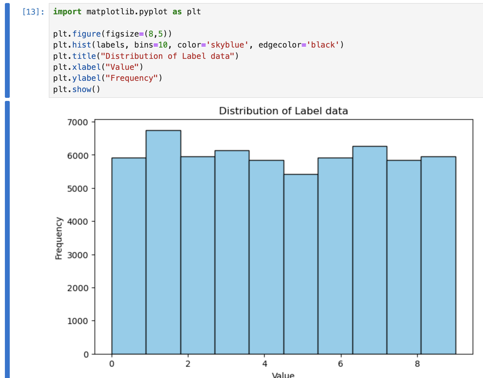
We can see a relatively even distribution for the data for each number.
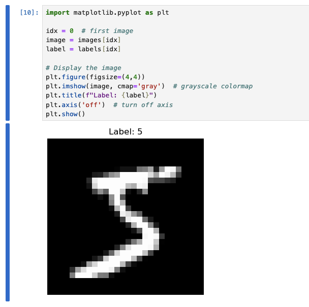
How about inspecting some of the images:
import matplotlib.pyplot as plt

idx = 0  # first image
image = images[idx]
label = labels[idx]

# Display the image
plt.figure(figsize=(4,4))
plt.imshow(image, cmap='gray')  # grayscale colormap
plt.title(f"Label: {label}")
plt.axis('off')  # turn off axis
plt.show()
Data ingestion pipeline
At this point, I’m not entirely sure if using Airflow here will be overkill… but I want to understand how this fits into a more “real” setup, not just a notebook, so let’s give it a go.
We’ll start with a small DAG pipeline that can process what we have done so far:
- Obtain data
- Convert into managable
We’ll create a slightly more dynamic script for performing the conversion:
from airflow import DAG
from airflow.operators.python import PythonOperator
from datetime import datetime
import os
import urllib.request
import subprocess
import struct
import numpy as np
import gzip
import h5py

RAW_DIR = "/opt/airflow/dags/data/raw"
PROCESSED_DIR = "/opt/airflow/dags/data/processed"

MNIST_URLS = {
    "train-images-idx3-ubyte.gz": "https://github.com/hamlinzheng/mnist/raw/refs/heads/master/dataset/train-images-idx3-ubyte.gz",
    "train-labels-idx1-ubyte.gz": "https://github.com/hamlinzheng/mnist/raw/refs/heads/master/dataset/train-labels-idx1-ubyte.gz",
}


def download_data():
    os.makedirs(RAW_DIR, exist_ok=True)

    for filename, url in MNIST_URLS.items():
        filepath = os.path.join(RAW_DIR, filename)

        if not os.path.exists(filepath):
            print(f"Downloading {filename}...")
            urllib.request.urlretrieve(url, filepath)
        else:
            print(f"{filename} already exists, skipping.")


def load_images(path):
    with gzip.open(path, 'rb') as f:
        _, num, rows, cols = struct.unpack(">IIII", f.read(16))
        data = np.frombuffer(f.read(), dtype=np.uint8)
        return data.reshape(num, rows, cols)


def load_labels(path):
    with gzip.open(path, 'rb') as f:
        _, num = struct.unpack(">II", f.read(8))
        return np.frombuffer(f.read(), dtype=np.uint8)


def convert_data():
    os.makedirs(PROCESSED_DIR, exist_ok=True)

    images = load_images(os.path.join(RAW_DIR, "train-images-idx3-ubyte.gz"))
    labels = load_labels(os.path.join(RAW_DIR, "train-labels-idx1-ubyte.gz"))

    output_path = os.path.join(PROCESSED_DIR, "mnist.h5")

    with h5py.File(output_path, "w") as f:
        f.create_dataset("images", data=images, compression="gzip")
        f.create_dataset("labels", data=labels, compression="gzip")

    print(f"Saved dataset to {output_path}")


with DAG(
    dag_id="mnist_pipeline",
    start_date=datetime(2024, 1, 1),
    schedule_interval=None,
    catchup=False,
    tags=["ml", "mnist"],
) as dag:

    download_task = PythonOperator(
        task_id="download_mnist",
        python_callable=download_data,
    )

    convert_task = PythonOperator(
        task_id="convert_to_hdf5",
        python_callable=convert_data,
    )

    download_task >> convert_task
Then execute using the following:
import requests
import json

AIRFLOW_URL = "http://airflow:8080/api/v1"
DAG_ID = "mnist_pipeline"
USERNAME = "airflow"
PASSWORD = "airflow"

payload = {
    "conf": {}
}

response = requests.post(
    f"{AIRFLOW_URL}/dags/{DAG_ID}/dagRuns",
    auth=(USERNAME, PASSWORD),
    headers={"Content-Type": "application/json"},
    data=json.dumps(payload)
)

print(response.status_code, response.json())
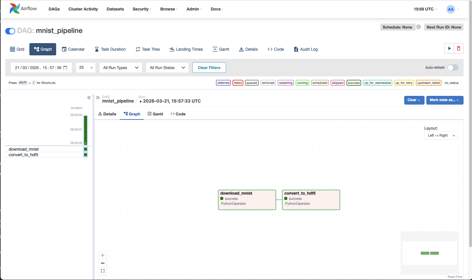
Now we have data in ./data/pocessed!
notes
Whilst trying to run this, I saw three issues (all fixed in the above docker-compose):
- Authentication wasn’t working - a user needed to be created - apparently the default airflow:airflow didn’t work
- Mapping the dags directly directly to the wokspace wasn’t ideal, as it mixed things up a lot.
Instead, mapping the workspace to a workspace directory inside airflow and then setting the env variable to look for a dags subdirectory helped organise things a lot.Instead, mapping exactly the same container path in airflow mean that any absolute directories were identical in both :sigh: - Linking the containers to allow DNS resolution was much easier :D
But also: airflow didn’t contain the required packages I needed (h5py) and errored during startup because of the DAG code. To combat this, performing a simple build of a custom docker image, which just performed a pip install appeared to help… but I ran into:
airflow | ValueError: numpy.dtype size changed, may indicate binary incompatibility. Expected 96 from C header, got 88 from PyObject
Whilst unfortunate, installing h5py with --no-deps did fix it, I wouldn’t recommend it.. probably safest would have been to dump the installed packages, add h5py and install the lot - at least this way pre-install packages would have been taken into consideration as dependencies rather than steamrolling all over them.
So little Dockerfile.airflow later:
FROM apache/airflow:2.8.3-python3.11

# Install h5py
RUN pip install --no-deps h5py
and a little:
@@ -14,7 +14,9 @@
     ports:
       - "5432:5432"
   airflow:
-    image: apache/airflow:2.8.3-python3.11
+    build:
+      context: .
+      dockerfile: Dockerfile.airflow
     container_name: airflow
     restart: always
     environment:
and all starts with no errors.
And, honestly, I couldn’t be bothered to get authentication working, so just run:
docker exec airflow airflow users create --role Admin --username airflow --email airflow --firstname airflow --lastname airflow --password airflow
Blame PEBKAC or airflow docs, but :shrug: it works.
Neutral Network
Next we’ll take a look at the basis of a neural network - my basic understanding is currently just:
Input -> Hidden Layers -> Output
We have our inputs (rows * columns * colour depth) of pixels to provide the image to the model.
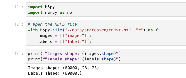
Loading data
Let’s first read in our data using the new format and validate it:
import h5py
import numpy as np

with h5py.File("./data/processed/mnist.h5", "r") as f:
    images = f["images"][:]
    labels = f["labels"][:]
To be able to work with the default Jupyter image, I had to install tensorflow. The options are either install in a terminal or build a custom iamge that installs it on top. On top of this, due to cross-dependencies, I had various issues, so pinning tensorflow and numpy worked for me:
pip install tensorflow=2.13 h5py=3.10 numpy=1.24.3
Organising data
Let’s first gear our data to be suitable for the inputs - we no longer care about the magical 2-dimensions of images, so we’ll have a set of 1-dimensional pixel values. Since everything surrounding neurons in ML is floats between 0 and 1, we’ll need to convert them to be between these values.
Looking at the shapes of the data that we have:

We can use this to reshape the image data into a 2-dimensional array:
x_shaped = images.reshape(images.shape[0], -1)

X = x_shaped.astype("float32") / 255.0
y = labels.astype("int64")
The thing to note here is that images.reshape is taking the shape of outer dimension of our data (the number of images), so 60000 and then telling it to reshape that data based on this and then -1 is telling it to “go figure it out”, so it’s effectively flattening the x/y dimensions into a single dimension of pixels. Realistically, no different to using x_shaped = images.reshape(images.shape[0], 28*28). We are then converting all of the values into floats (for the input data) and dividing by the pixel color depth (which is 1 byte), translating it from 0-255 -> 0-1.
Next, we will do two things, shuffle the data so it’s in a random order (though it may well be already) and then split into two sets:
- The first set we’ll use to train the model
- The second set will be used to test the model
This separation is very important - if we test our model against the data that we used to train it, we’ll not proving that it can reliably convert generic images, just that it is able to recognise this set of images. Whilst the original data did provide a seperate set of training and test images, it was just easier to deal with fewer files and, in a real world scenario, we would just have some source data - both need labelling/categorising and we’d likely have to split it like this anyway, so I think this is fine and probably more of a real-world example
# Number of elements from the outer shape (as we can see above)
num_samples = X.shape[0]

indices = np.arange(num_samples)

# We'll use the seed with a static number - in most situations this is awful, but for our use-case have a re-producable result is idea,
# if anything because it means we can debug the script in jupyter more easily.
np.random.seed(42)
np.random.shuffle(indices)

# Split total number of samples by an 80:20 split of training vs test data
split_idx = int(0.8 * num_samples)
train_idx = indices[:split_idx]
test_idx = indices[split_idx:]

# We'll then index the actual data, splitting it into the training/test data
# Note that because train_idx/test_idx are a set of indices, we can easily split both the image data and the labels, so we can
# retain the relationship between them, both in the split and the shuffle, which is obviously vital
X_train, y_train = X[train_idx], y[train_idx]
X_test, y_test = X[test_idx], y[test_idx]

# Verify the number of elements in our test/train data
print(f"Train: {X_train.shape}, Test: {X_test.shape}")
# > Train: (48000, 784), Test: (12000, 784)
Creating the model
Now we get into the territory of “omg, what is that”… I’m going to start with what we see in tutorials and then try to break it down:
import tensorflow as tf
from tensorflow.keras.models import Sequential
from tensorflow.keras.layers import Dense, Input

model = Sequential([
    Input(shape=(784,)),       # input layer, flattened images
    Dense(128, activation='relu'),  # first hidden layer
    Dense(64, activation='relu'),   # second hidden layer
    Dense(10, activation='softmax') # output layer (10 digits)
])

# Compile with optimizer + loss
model.compile(
    optimizer=tf.keras.optimizers.Adam(learning_rate=0.001),
    loss='sparse_categorical_crossentropy',  # labels are integers
    metrics=['accuracy']
)

model.summary()
# Model: "sequential"
# _________________________________________________________________
#  Layer (type)                Output Shape              Param #
# =================================================================
#  dense (Dense)               (None, 128)               100480
#
#  dense_1 (Dense)             (None, 64)                8256
#
#  dense_2 (Dense)             (None, 10)                650
#
# =================================================================
# Total params: 109386 (427.29 KB)
# Trainable params: 109386 (427.29 KB)
# Non-trainable params: 0 (0.00 Byte)
# _________________________________________________________________
We start by intialising a Sequential object, a Keras model, which is basically a container for a set of layers.
This is the entity that will control training, evaluation and can be used to save/loaded (we’ll go into this later).
In this example we are initialising the whole thing in the constructor, but can equally do:
model = Sequential()
model.add(Input(...))
model.add(...)
Walking through the layers that we’re adding to our model:
Input layer
Input(shape=(784,))
This is quite simply defining the input layer and the shape, as we’ve seen, is the shape of our pixel data.
Dense (hidden) layers
Dense(X, activation='relu')
This is defining our first and second hidden layers.
A dense layer is basically taking every input value, connect it to every neuron in this layer, multiply by weights, add bias, then apply an activation function.
Using Dense(128), we are creating:
- 128 neurons (as defined in the parameter)
- Each neuron has:
- 784 weights (based on a connection to each of the 784 inputs)
- 1 bias
The next layer will then contain the number of neurons that we specify, but each neuron will contain a “connection” and associated weight to each of the neurons in the previous layer.
Imagine a big list of neurons. Each neuron has a weight for every connection to the neurons in the next layer. To get the output, each neuron multiplies its input by its weight, sums them up with a bias, and applies an activation function.
A suggested rule of thumb for the size of these layers appears to be:
| Layer size | Meaning |
|---|---|
| Too small | Not enough capacity -> underfitting |
| Too big | Overfits + slow |
| Medium (64–512) | Good starting point |
For the dataset that we have, the suggestion is: For MNIST:
- ~128 for the first layer
- 64 and down for following layers, which gradually compresses the “features” of the input data, e.g. 784 (our inputs) -> 128 -> 64 -> 10 (our outputs)
Activation
So far, I’ve imagined the layers as (what I’ve been told is) flat algebraic equations, that is:
Input @ Weight + b
So we multiply the input of the neuron by its weight, sum them, and add the bias. However, what happens is after this an activation function is used. Activation functions introduce non-linearity, which lets the network model detect complex patterns. Without activations, the network can only separate data using straight lines.
This is one of the things, for me, that I’m just going to have to accept for now.
In this example we’re using ReLU, which is very simple:
f(x) = max(0, x)
Meaning we’re putting a lower bound on the output to 0. It’s a very cheap calculation and avoids the “vanishing gradient”.
Other alternatives are:
- Sigmoid -
f(x) = 1 / (1 + e^-x), which provides a 0→1 output, but it’s slow and doesn’t avoid vanishing gradients. Useful for binary classification output. - Tanh - Provides a zero-centred output, i.e. -1 → 1.
- Softmax (which we’re using in the output layer) - Converts outputs into probabilities:
[2.1, 1.3, 0.2, ...] -> [0.65, 0.2, 0.02, ...]
The sum of the outputs is 1 and can be used for representing confidence per class.
What are vanishing gradients?
First we need to talk about loss — we can think about loss simply as “how wrong the network is”. Using ours as an example, we have a given handwritten digit 2; the output for 2 will (hopefully) have the highest ratio in the last layer. All of the combined values in the incorrect outputs are considered loss.
For example:
[1: 0.1, 2: 0.8, 3: 0.1, ...] # our loss here is 0.2
We’ll get to how to deal with loss shortly, but simply, whilst training, the weight is calculated through:
weight(new) = weight(old) - η · (∂Loss / ∂W)
So:
Weight = weight - learningRate * (Loss / Weight)
If we always have an output capped to 1 (with the activation function), we will always have a weight that gradually reduces. So if we have multiple layers, the weights of the deeper layers can eventually get close to 0 — thus vanishing.
Why are “dense” layers used and what alternatives are there?
- Convolutional layers (Conv2D)
- Instead of: “connect everything to everything”, these will look at smaller groups of inputs together.
- This is better for edges (a place where pixel values change sharply), shapes and spatial patterns
- Imagine a tiny “filter neuron” (like a little stencil) with a small number of weights. This neuron slides over the image in a grid-like way, reusing the same weights everywhere. Each position it lands on, it multiplies the input pixels by the filter weights, sums them, and outputs one number. Stack a few filters, and you get a “feature map” that detects patterns like edges or shapes.
- Recurrent layers (LSTM / GRU)
- These are used for sequences, time-series and text
- These aren’t useful for interpretting pixels
- Imagine a neuron that can remember. It takes an input and its own previous state, multiplies them by weights, sums them, and produces a new state and output. This neuron is reused at every time step in a sequence.
- Transformer-style layers
- These are attention-based and used in modern AI
- Imagine a neuron that doesn’t just see one input at a time, but can look at all other neurons in the same layer and decide which ones are important. It uses multiple sets of weights (queries, keys, values) to “attend” to everything else, then combines that information to produce an output.
| Layer type | Think of it as | Key idea |
|---|---|---|
| Dense | Big wiring mess | Learn everything brute force |
| Conv2D | Sliding magnifying glass | Detect local patterns |
| RNN | Loop with memory | Process sequences step-by-step |
| Transformer | Group discussion | Everything attends to everything |
Compile
Next we’ll look at the compile call:
model.compile(
    optimizer=tf.keras.optimizers.Adam(learning_rate=0.001),
    loss='sparse_categorical_crossentropy',
    metrics=['accuracy'],
)
Optimis(z)er
During the first iteration of training, we can imagine the following occurs:
- All of the models weights/biases are random
- We pass in our first image to the input neurons.
- These go through the layers Input -> Hidden Layer(s).. -> Output
- The output is compaed against the expected value and the loss is calculated.
- Next, the network computes gradients: how much each weight and bias contributed to the loss. These gradients point in the direction that would reduce the loss if the weights changed.
- Finally, it is the optimiz(s)er’s responsibility to determine how to adjust all of the weights and biases based on the gradient.
We could imagine that if we blindly update weights and biases, we could end up easily going round in circles or getting exponentially large/small, so the optimiser does various things:
- Scales the update based on momentum (past gradients)
- Adjusts based on variance of gradients
- Potentially clips, normalizes, or smooths updates
In the example we’re specifying a tf.keras.optimizers.Adam optimiser.
Adam (short for Adaptive Moment Estimation) is a popular optimis(z)er because it:
- Combines the ideas of momentum (smooths out updates by remembering previous gradients) and adaptive learning rates (changes the step size for each weight based on how fast it’s changing).
- Often converges faster and more reliably than simpler methods.
What it does under the hood:
- Tracks moving averages of gradients – this is the “momentum” part.
- Adjusts the step size for each parameter individually – the “adaptive” part.
- Updates the weight with:
weight(new) = weight(old) - step_size * adjusted_gradient
This ensures weights move in the “right” direction efficiently without overshooting.
Some other optimizers include:
- SGD (Stochastic Gradient Descent) – the simplest one, updates weights along the negative gradient. Can be combined with momentum for better performance.
- RMSprop – keeps a moving average of squared gradients to normalize updates. Works well with recurrent networks.
- Adagrad – adapts the learning rate per parameter but can decay too aggressively.
Learning rate
This is very basically, what size steps should be taken whilst making adjustments.
If this is too small, training will take too long. If it’s too big, we can overshoot, weights bounce around, never settle.
We can probably think about this as a guessing game.. if I’m guessing a number between 1 and 100 and I get told if I’m too high or low. If I change 1 at a time, it will take a long time to find the number, if I jump 50 at a time, I’d not get a precise number and would never arive at the real number.
Considering this, the natural thought might be: can we start big and get smaller…
And they can, this is called decay, which can be found in adam and other optimis(z)ers
Loss
loss='sparse_categorical_crossentropy',
This parameter is telling the model how to measure the loss. If we imagine that “loss” is just a value that the optimiser is trying to reduce and the loss function is taking the state of the model during training to provide this value - so it’s this function that is reading the output values and comparing to the labels to give a loss value.
sparse_categorical_crossentropy is a commonly used for categorisation models (like ours) and allows the network to know how wrong it is and in which direction to adjust weights, without needing to encode labels as [0,0,1,0,...].
1. Categorical / Multi-class Classification
-
categorical_crossentropy- Used when your labels are one-hot encoded (e.g.,
[0, 0, 1, 0]). - Measures how different the predicted probabilities are from the true class distribution.
- Example: predicting digits 0–9 in MNIST.
- Used when your labels are one-hot encoded (e.g.,
-
sparse_categorical_crossentropy- Used when your labels are integers (e.g.,
2instead of[0,0,1,0,...]). - Internally converts integers to one-hot for the calculation.
- This is why it’s convenient for MNIST: labels are just numbers 0–9.
- Used when your labels are integers (e.g.,
2. Binary Classification
-
binary_crossentropy- Used when there are only two classes, e.g., spam vs. not spam.
- Output is a single probability (0–1).
- Measures how far the predicted probability is from the actual class.
3. Regression (continuous outputs)
-
mean_squared_error(MSE)- Measures the squared difference between predicted and true values.
- Common in predicting continuous numbers like house prices or temperatures.
- Penalizes large errors more than small ones.
-
mean_absolute_error(MAE)- Measures the absolute difference between predicted and true values.
- Less sensitive to outliers than MSE.
-
Huber loss- Combines MSE and MAE: small errors use squared difference, large errors use absolute difference.
- More robust than MSE if outliers exist.
4. Advanced / Special Cases
-
Kullback–Leibler Divergence (
kld)- Measures how one probability distribution differs from another.
- Useful in some probabilistic models or when distilling one network into another.
-
Contrastive / Triplet Loss
- Often used in embedding spaces (e.g., face recognition) to bring similar items closer and push dissimilar items apart.
Metrics
The final part of our model definition is metrics=['accuracy'],.
Metrics are purely for observability of our model, not for feedback for training (like the loss function).
accuracy will tell us the fraction of correct predictions.
-
Binary classification:
binary_accuracy,AUC,Precision,Recall,F1-score
-
Multi-class classification:
categorical_accuracy,top_k_categorical_accuracy(useful if you want the correct class in the top K predictions)
-
Regression:
mean_absolute_error,mean_squared_error,root_mean_squared_error,R^2
TRAINING OUR MODEL!!
Saving the model
The model can be saved and later loaded, this will contain:
- Weights and Biases (the results of our training)
- The model architecture, i.e. Layer definitions and how they are connected
- Optimiser state:
- The optimiser itself (e.g. Adam)
- Learning rate
- Internal optimiser state (momentum, etc.)
Using this, we should be able to save the whole thing and then load it simply into a model object and run inference:
model.save("model.keras")

loaded_model = tf.keras.models.load_model("model.keras")
# @TODO Run inference here...
More Definitions
- Feed Forward networks
- Convolutional Neural Networks (CNNs)
- Recurrent Neural Networks (RNNs)
- Generative Adversarial Networks (GANs) Autoencoders
- Transformer networks